Analyzing and understanding funnels is an essential skill for every product manager (PM). It helps them to understand and optimize product and feature usage, by enabling them to track and visualize the customer journey from acquisition, through activation, retention, referral, and revenue; or user sub-journeys through any workflow in the product – while highlighting conversion and drop-off rates along the way. Using funnel analysis, PMs can define any success criteria and track the steps a user takes to reach the success criteria in case of conversion, or the point in the product where the user aborted the workflow, in the case of a drop-off.
This kind of analysis is quite different from business analytics, which aggregates measures on a set of dimensional attributes to understand business outcomes. However, based on my 10+ years of experience building high-performance databases, I believe that modern data warehouses are well equipped to efficiently execute such (in fact, all product analytics) workloads at scale. You can read more about that here.
In this post, I’ll dive deep into the internals of the computation that goes behind calculating funnels, and detail how modern data warehouses can execute funnel queries at scale.
What is Funnel Analysis?
Wikipedia defines funnel analysis as mapping and analyzing a series of events that lead towards a defined goal, like an advertisement-to-purchase journey in online advertising. The example below follows the conversion of users to “Paid Activation” after taking training courses on an online learning platform – 18.6% of users take the “Analytics Course” after “Getting Started”; and of those, 31% of users convert to “Paid Activation”, for a total conversion of 5.8%.
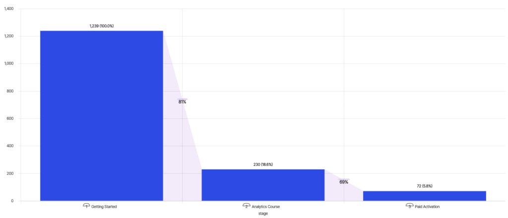
A PM looking to increase engagement can look at conversion and drop-off rates between various stages and decide to focus on improving the conversion between “Getting Started” and “Analytics Course” to increase “Paid Activation”.
How to Build a Funnel
Conceptually, a funnel follows an ordered sequence of events by “event_time” for each user to calculate the farthest funnel stage they reached. There are multiple ways to express this calculation using SQL. We’ll cover two such patterns and provide insights into the performance for both. But before jumping to SQL, let us concretely define the data model used for this analysis.
Data Model
Let us assume a schema with a single “Events” table. The data in “Events” can be imagined to have the following shape:
I have made two simplifying assumptions in this model, however as I explain below, neither of these assumptions is an area of concern for modern data warehouses.
- Structured Data – “Events” is assumed to be a structured table even though event data is almost always semi-structured. Refer to my previous blog to understand how data warehouses handle semi-structured data efficiently.
- No Joins – First-generation tools like Amplitude and Mixpanel model their schema as a single event stream. This model can be highly restrictive, especially since any real-world analysis requires business context from other sources. Unlike first-generation product analytics tools like Amplitude and Mixpanel, which provide extremely limited querying capabilities, modern data warehouses are built to join multiple tables efficiently.
Funnel Query
Query engines parse and optimize SQL text to create an optimized relational plan for execution. Let us visualize the optimized relational plan for this SQL to better understand its execution profile. There is one subquery for each stage of the funnel:
- stage1 subquery emits unique user_ids that encountered the “Getting Started” event
- stage2 subquery joins the “Events” table with stage1 output to emit individual user_ids that reached the “Analytics Course” event after “Getting Started” event
- stage3 subquery joins the “Events” table with stage2 output to emit unique user_ids that reached “Paid Activation” event after the “Getting Started” and “Analytics Course” event, in that order
- Output from all three stages is aggregated to count the number of unique users in each stage
Modern data warehouses have extremely sophisticated query planners to optimize relational trees. There are two optimizations in the plan above that are worth calling out:
- Computation for each stage happens once – The optimizer factors out redundant computations in the plan as sub-plans or fragments to reuse results across the query. Best-in-class engines schedule sub-plans adaptively to use results and statistics for further planning.
- Aggregation in the “Final Output” is pushed below the join – Best-in-class optimizers should be able to infer that aggregate can be pushed below the left join for many-to-one join, like here, to eliminate the cost of expensive left join between the three stages. Crafting a query that aggregates before joining is also a viable option for an analytics engine in case the optimizer is unable to optimize for this pattern.
Aggregate and Join operations are bread-and-butter for modern data warehouses, allowing such queries to be executed efficiently at scale with massive parallelism. However, there are still a couple of improvements that can further improve query performance:
- Join between subqueries – Join between subqueries are more expensive than base table joins since subqueries do not have join indices precomputed. In our example, “Events” and each stage output are joined at user grain, which can be costly for high cardinality users. Note that the cross-join in the final query is pretty cheap since it joins precisely one row from each input.
- Multiple scans – Even after removing redundant computation, the “Events” table is scanned three times, one for each subquery. A faster, more efficient algorithm would scan the “Events” table just once.
Stacked Window Functions Query
An alternate approach to declare this computation is using window functions. Window functions enable imperative event sequence style analysis via the declarative SQL interface. In this approach, we create a stack of window functions (partition over), one for each stage in the funnel, followed by a count distinct of “user_ids” at the top of this stack. We call this pattern the Stacked Window Functions pattern. Here’s the SQL for creating the same funnel using Stacked Window Functions.
Though the above query is more verbose, it creates a much simpler relational plan – most of the complexity for calculating the funnel is pushed inside the window function.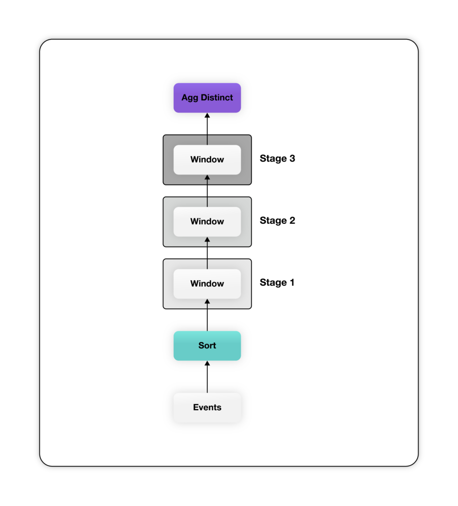 The plan above has one window function for every stage of the funnel. Notice that the window functions defined in the SQL code above partitions its input by “user_id” and orders by “event_time” to ensure that data for each user is processed by the same window function instance in the increasing order of “event_time”. Each window function emits an extra column containing the earliest timestamp when the user reaches the corresponding stage, or null if the user doesn’t reach that stage. Finally, the output from the last window, containing one column with “event_time” for each stage for all users, is aggregated to count distinct “user_ids” per stage.
Like before, the query planner in most modern data warehouses makes two critical optimizations for improved performance of the above plan:
- Single Sort across Windows – All window functions are partitioned on “user_id” and sorted on “event_time”. In such a case, the optimizer creates a single sort operator that feeds data in the desired order to all window functions.
- Local distinct aggregation – The query has a distinct aggregation on “user_id”. This aggregation can be performed within a partition (locally) if data is pre-partitioned on “user_id” since user-based partitioning guarantees that users will not need to be aggregated across partitions.
Both the optimizations listed above are standard in most modern data warehouses. This formulation of funnel query doesn’t have either of the shortcomings of the Join Sequence style of funnel query. However, there is one problem that needs to be addressed. The Sort operator atop the Events scan may seem expensive to compute. Fortunately, this sort isn’t required to be global; sorting locally within the partition is sufficient since the window operator requires sorted input per user and not across users.
There is potential to optimize this query every further. Most data warehouses offer a knob to cluster tables using a user-provided Clustering Key. Clustering Key is a set of columns or column expressions used to colocate rows of a table close to each other for improved performance. Clustering the “Events” table by “event_time” has multiple advantages:
- Reduce (may even eliminate) the cost of Sort operator if the data is almost (or fully) sorted by event time
- Improve scan performance on “Events” for queries with time range filters on “event_time” column
Conclusion
In this blog, we presented two different formulations of funnel analysis SQL and analyzed their respective query plans to understand their performance profile in modern data warehouses.
First-generation tools, like Mixpanel and Amplitude, have an outdated architecture that requires data movement, creates data silos and duplication, and is also prohibitively expensive at scale. Modern data warehouses have matured to a point where they can natively provide an interactive experience for product analytics workloads without these shortcomings and the flexibility of tunable cost for desirable performance.
NetSpring can connect to all major cloud data warehouse vendors, including Snowflake, BigQuery, Redshift, and Databricks to provide a rich product analytics experience – without any data movement and at a third of the cost of legacy approaches. Request a demo today!